From Smith, Howard M., Principles of Holography, 2nd. Edition, John Wiley & Sons, New York, 1975, p. 174.. ISBN 0-471-80341-3
I became intimately familiar with what was known as the "Benton Math" while designing Holographic Optical Elements as a Research Associate at Lake Forest College. In his seminal papers at the LFC ISDH's of 1982 and 1985, Dr. Stephen Benton, inventor of the white light transmission hologram, or rainbow hologram, or Benton Hologram, revealed to the world of holographers the "shop math" necessary to accurately register colors in his recording regime, and why it works that way, and that it's not that difficult to figure out on your own. It could be argued that these fundamental equations should not be denoted with any one person's name, as they all can be derived by the enthusiastic holographic geometer from the basic diffraction equations. But Benton's genius was in the application and explication so that the typical bargain basement holographer could follow his Euclidean exposition.
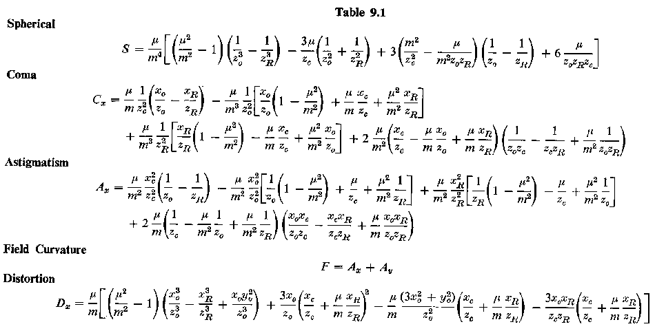
For instance, instead of this,
From Smith, Howard M., Principles of Holography, 2nd. Edition, John Wiley & Sons, New York, 1975, p. 174.. ISBN 0-471-80341-3
Benton gives us this:
From Benton, S. A., The Mathematical Optcs of Whitel-light Transmission Holograms, Proceedings of the International Symposium on Display Holography, Volume, T. Jeong, editor, Lake Forest College Press, 1983. Available here and here.
In the common holographer’s lexicon these calculations became known as the Benton Math, viz. the cover of this issue of holosphere.
Besides calculating slit parameters, these generalized equations can calculate point source parameters. And I was using them to design Holographic Optical Elements for laboratory instruments under a grant from a major medical equipment manufacturer. (The basic concept of the diagnostic device that utilized the HOE would be to measure one or two wavelengths of interest of an interrogating light source, passing through a reagent that had been mixed with a sample from a patient. A dedicated spectrophotometer for urine testing perhaps, as most of the calibration test samples were yellowy.)
Sitting down with a calculator and a pad of graph paper and a hot cup of Joe I was running the numbers and seeing what happens if something is here and where does the light end up. Three sets of calculations needed to be run: the first one to find the new output angle, if there is a wavelength change, and use that to find the s (sagittal) and t (transverse) foci. Vertical and horizontal foci are terms that could be substituted for s and t, however the former are absolute orientations, while the s and t relate to the planes the beams enter as seen by the holographic plate or lens as illustrated below.
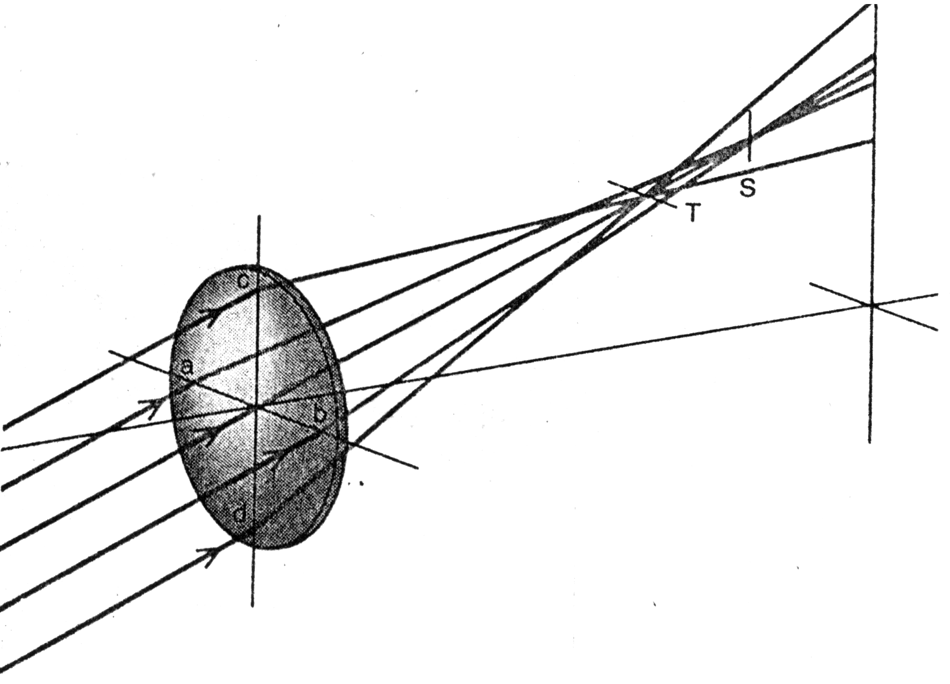
To complicate matters of terminology, most of the time the rainbow holograms are recorded on an optical table with the geometry turned sideways for added stability, instead of growing taller and shakier; the reference beam is horizontal during recording, but will be rotated 90 degrees during reconstruction, illuminating in the vertical plane, typically from the top, but sometimes from below. (Rainbow holograms won’t work with side references; you will see why by the end of the article.) The picture above, illustrating astigmatism from an object point below the optical axis of the lens, could be also illustrating the two real astigmatic foci of an object point from a circularly shaped hologram.
Flipping the image over to orient the rays to the more common top replay case looks like this:
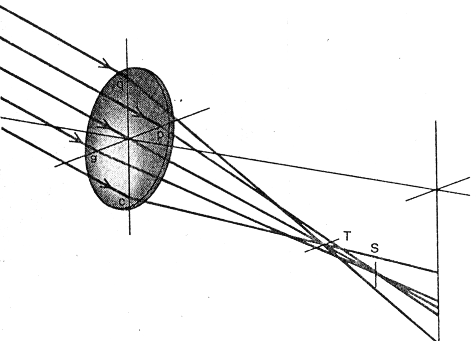
The horizontal line at T is not the Horizontal Focus; it is the Vertical Focus, as the rays in the vertical plane are converging. S is the Horizontal Focus, as it is narrowest in that plane, caused by horizontal rays converging.
Ray tracing two coordinates on graph paper (with colored pencils in some cases!) leaves a little to be desired for the three-dimensional mind to visualize. So I decided to make a grating to a simple prescription and make a graph to 1:1 scale and see if the rays coming out of the grating lineup with the colored pencils! (Although this write up is being posted in 2015, this research was done in 1990, way before computers were as ubiquitous as today!)
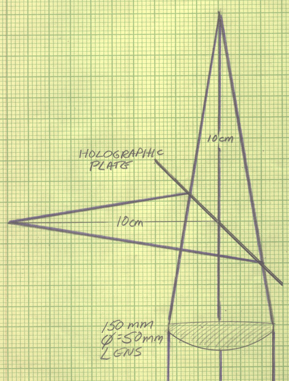
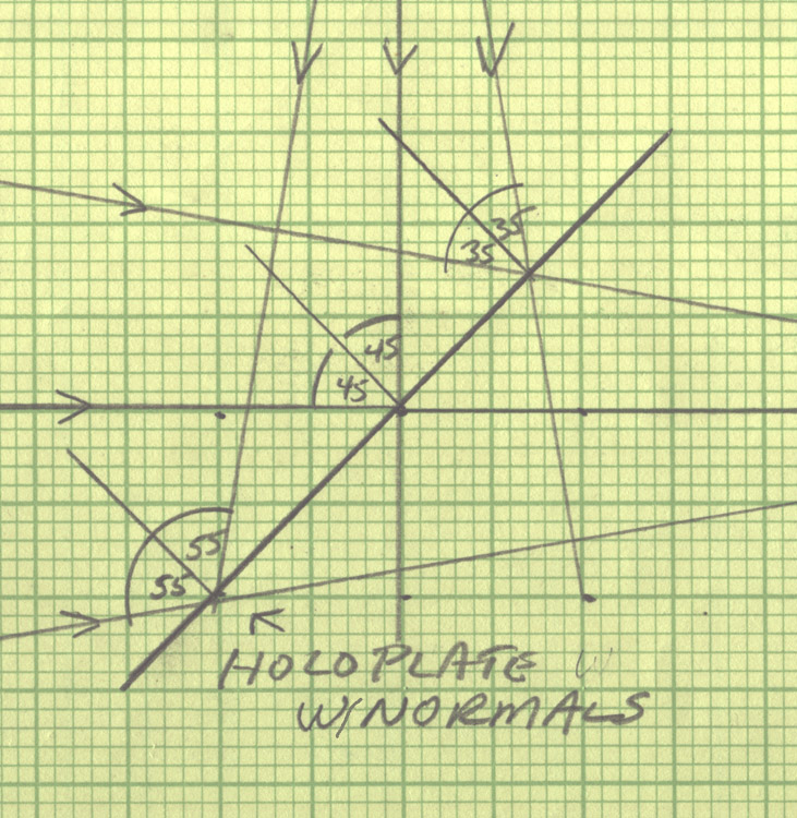
The HOE prescription was what I called a 10 cm by 10 cm grating. Both of the beams were incident on the holoplate at 45 degrees from the normal, with one of them diverging from a point 10 cm away from the center of the plate, the other converging 10 cm beyond the plate, first schematically, then practically:
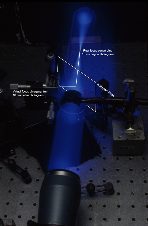
476 nm photons illuminate the recording geometry.
A note about the photographs above and below: The web page images were scanned in from Ektachrome color slides shot at the time of the experiment (1990). A few Photoshop adjustments were made for better photographic rendering, but the beams were “painted in” in the original film photographs by setting up the shot with the camera on a tripod, opening its shutter with the room lights out, and passing a sheet of Kodak Lens Cleaning Tissue through the beams so that the dot on the paper averages into the beam streaks. Then the electronic flash was fired, usually a stop or two or three underexposed so that the stainless steel tabletop backdrop doesn’t overwhelm the beam. This works with the diverging, collimated, and converging beams, too, as evidenced in the figure which is the piece de resistance of this magnum opus further below!
The back end of the table set up prior to this is in the best Mach-Zehnder interferometer tradition, a rectangular configuration, with a broadband polarizing beamsplitting cube in the kitty-corner from the holoplateholder, and the necessary half-wave plates to rectify the polarization vectors. There is one in each of the two beampaths, as mica half-wave retardation plates were used, which are somewhat broadband, but both of them were aligned to interfere with each other for each recording wavelength.
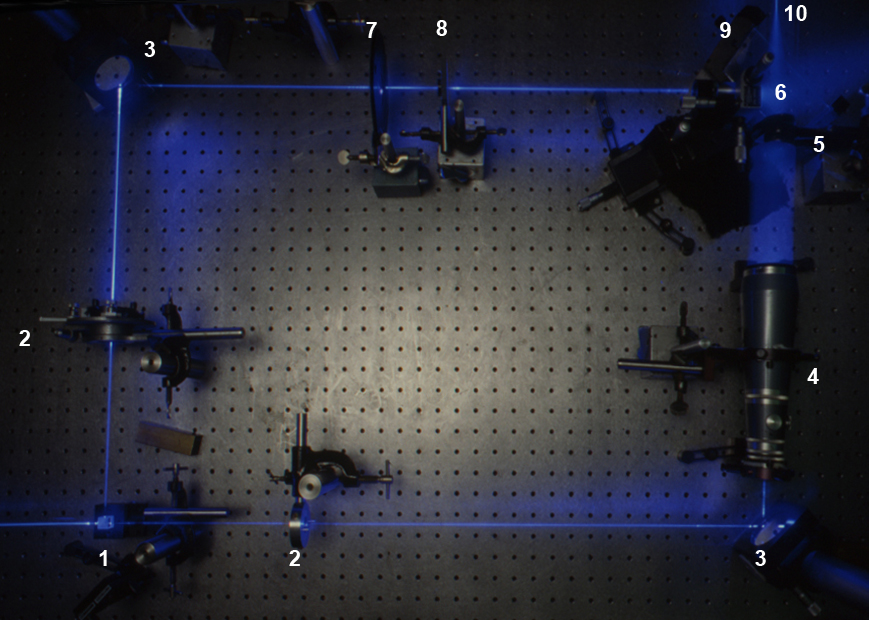
Legend:
#1 = Polarizing Beamsplitting Cube #2 = Half-Wave Retardation Plates #3 = Beam Steering Mirrors #4 = Spatial Filter/Collimator Assembly #5 = 125 mm Focal Length, 50 mm Aperture Achromat Lens #6 = 4” X 5” Plateholder #7 = Negative 100 mm Focal Length Lens (to pre-spread the beam before the spatial filter.) #8 = Iris Diaphragm #9 = Spatial Filter with 60X Objective on translating stages for accurate focus distance. #10 = Focus of #7, 10 cm beyond center of hologram.
These wavelengths were, to wit, 458, 476, 488, 496 and 515 emitted from the argon laser, (the 502 nm being too weak for this work) and the traditional 633 nm from the Helium-Neon.
Photons were supplied by a Coherent CR-2 Super Graphite Argon Laser, (graphite being part of the resonator structure, not for gain medium, for allegedly better stability?). It could be run single frequency or multi-line at the drop of a bayonet mounted mirror assembly, which made it invaluable for this dissertation. A translating mirror allowed a Jodon 1576 He-Ne (15 mW power, from a 76 cm cavity) to be injected into the set up if desired.
The HOE’s were recorded mainly on Agfa 8E materials, as the Ilford materials at that date had BIPS (Built-In Pre-Swell) to shift the replay wavelength of a reflection hologram to a shorter wavelength, a mis-guided marketing move if I ever saw one, as this concept might be OK for a red reflection recording regime, but for a green material not such a great idea! Its effect on transmission holograms tilts the fringes so that the reference beam for the brightest replay does not occur at the recording wavelength. (In which direction is the tilt is a problem left for the student.)
Solutions for this conceptual defect would be to simply wash out the BIPS in running water, soak in Ilfotol (Ilford’s answer Kodak’s Photo-Flo 200, and for 50 holographic recording materials trivia points, what was Agfa’s wetting agent called?) and dry, all in the dark. Another opportunity to ruin the plate, even before exposure. (Almost as many holograms are lost to drying issues as movement!) Not a practice I condone or tolerate if I have to.
My solution to this Ilford problem was to develop in a pyrogallol based solution to tan the gelatin for structural rigidity while it is expanded and wet, and follow it with not a reversal bleach but a rehalogenating bleach which also has tanning action. The success of this technique depends on developed density, so there is an optimum exposure/development combination that faithfully records the fringe system, over- or under-done holograms would reconstruct at less than or greater than their recording angles. Usually it works out that the best exposure is on-angle and the brightest of the bunch, but don’t depend on it.
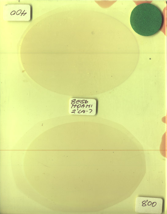
The appropriate Agfa 8E material was exposed, (‘75HD for the red, ‘56HD for the blues and greens, with the best results obtained on some 8E56HD AHI, {for Anti-Halation Intra-emulsion, an anti-scattering dye, which helped significantly} and maybe even some green exposures were made on red plates), developed for 2’ in CWC2 and bleached in CWPBQ2. Very bright, non-shifted fringe HOE’s were recorded 2 to a 4” by 5” plate by rotating the plate 180 degrees between exposures.
Plates had a peel off anti-halation backing applied to them thanks to the Universal Photonics X-59 Strip Coat brush on black coating for broadband protection for the elimination of the dreaded woodgrain.
The parameters involved in solving the "Benton equations" (or anybody else's holographic ones) are the recording wavelength, λ1, the angles of incidence of both of the interfering beams, θref and θobj, and the distances that both of the point sources are located from the holographic plate, Rref and Robj during recording. The distances are labelled R as they are measured radially, as spherical wavefronts are being discussed.In the case of recording the example HOE, θref = θobj = 45°, and Rref = Robj = 10 centimeters, but one is "behind" the plate (the one from the spatial filter) while the other is "in front", the real image formed by a lens 10 cm beyond the plate. Addition is changed to subtraction and vice versa while solving Benton's ARISTOTELIAN EQUATIONS OF HOLOGRAPHY to accommodate the signing convention.
The parameters involved in solving the "Benton equations" during relay are the replay wavelength, λ2, (for white light illumination a few iterations may need to be run), the angles of the illuminating beam, θill and of the exiting beam, θout, plus the distances that both of the point sources are located from the holographic plate during replay, Rill and Rout during recording. The distances are labeled R again. Usually it is θout and two of the Rout that are to be solved for, as there are horizontal and vertical foci due to the astigmatism inherent in the holographic recording. The following goes into excruciating detail on how the example holograms were characterized.
The first equation to be solved is the Diffraction Angle of the output beam, which relates the recording and replay wavelengths to the sines of the angles of reference, object and illumination. Here are the mind-numbing hand written solutions for the example HOE, as it were repositioned in the plateholder where it had been shot, so that the θill and Rill are the same as θref and Rref during recording. The θout is solely determined by the wavelength change. (HOE recorded at 515 nm, replay calculations at the other Argon laser lines of 496, 488, 476, and 458 nm.) (It's a good idea to run through the equation without changing the wavelength to see if your sign convention agrees with the ARISTOTELIAN EQUATIONS's)
Then the horizontal or y-focus distance is calculated, and it is only wavelength dependent again thanks to the in-situ interrogation. This distance is measured along the ray exiting the HOE at the previously calculated diffraction angle.
The most difficult is last, as it requires the diffraction angle of the first equation and the horizontal focus distance of the second to be solved. Plus it relies on the cosine of the angles squared! But it's not insurmountable.
Similar equations were solved for an HOE recorded at 488, and replayed with the panoply of wavelengths, and then graphed.
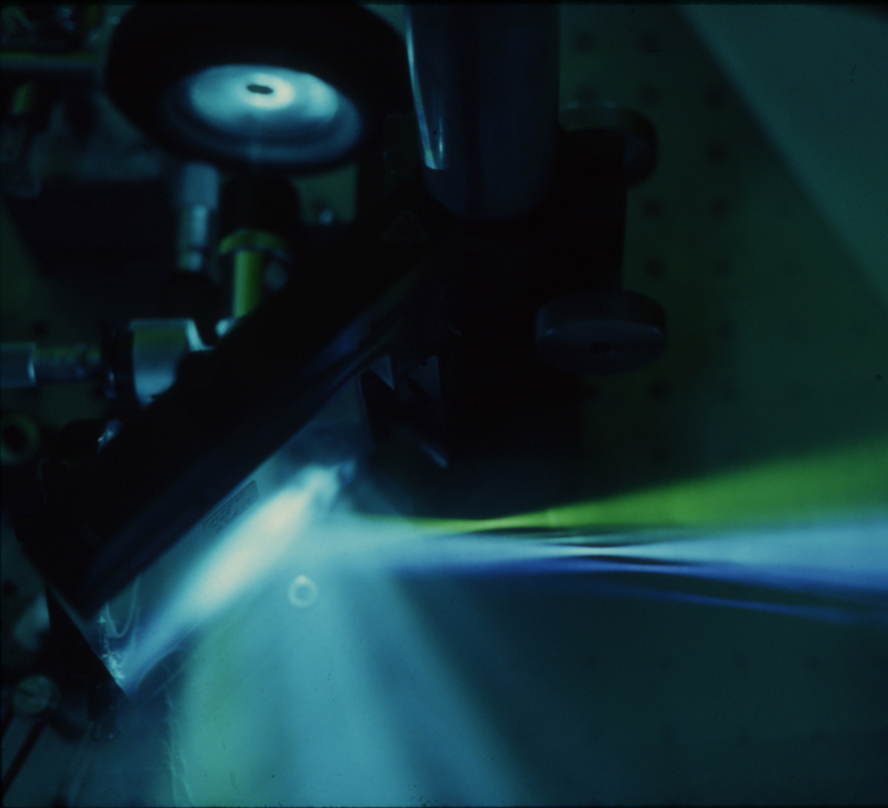
Here is the piece de resistance of this précis; the 10 by 10 cm HOE recorded at 488 nm, reconstructed by multi-line Argon laser photons. The reference spatial filter is diverging downward in the photograph, simulating a top lit hologram. The diffracted wavefronts travel to the right and focus, just like the sketch above.
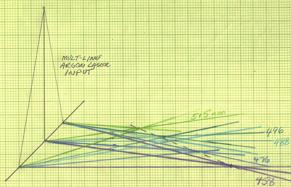
Below is the HOE recorded at 458 nm replayed with the multi-line argon laser. Notice that all the longer wavelengths are diffracted at larger angles.
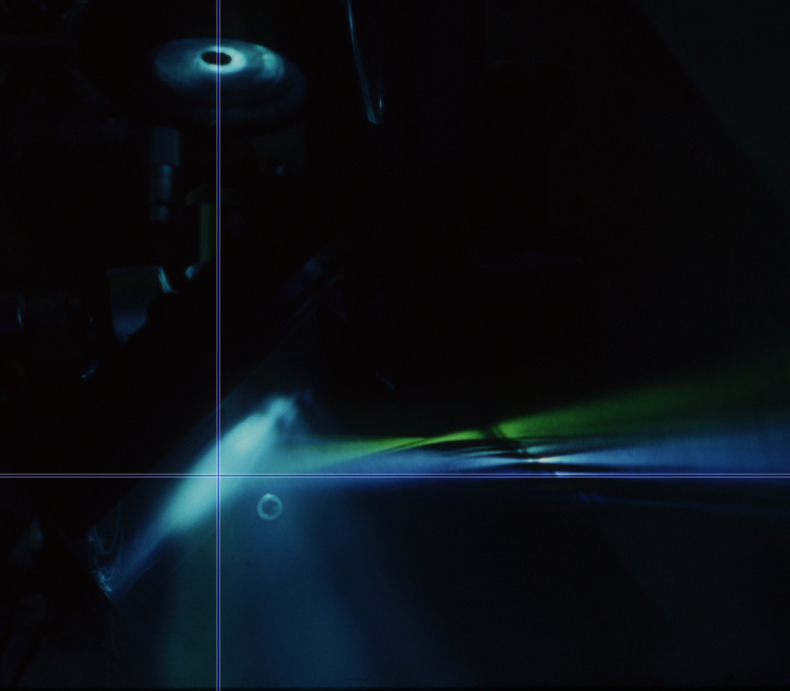
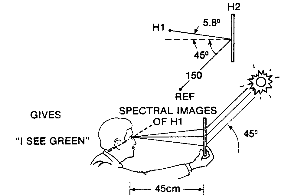
The above photos were taken from the vantage point of looking at the ray trace from the side, like the Benton “I see green!” illustration at the top of the page. These are the vertical foci, or T for Tangential. The picture below was taken in a plane at right angles to those above, like looking down on the hologram being replayed from the reference beam’s viewpoint. These are the horizontal foci, or S for Sagittal, and the only position where the T and S locations are the same is for the case when the illuminating wavelength is the same the recording one.
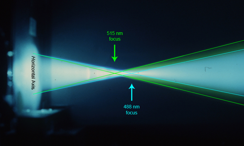
Another way of relating the viewpoints of the two sets of pictures is that the camera was placed above the optical table in the first set, (vertical or T foci) and in the second viewpoint the camera is on the tabletop, looking across at the horizontal focus. The hologram is placed in its plateholder with its horizontal axis vertically oriented in the photo. Yet another mind's eye conception of where this observation is taking place is that the camera is looking up from the floor at a top lit rainbow hologram. Only the two strongest Argon Laser emissions are decently exposed in this image, taken decades before the immediate gratification of exposure checking capability of the digital camera era, which helps to make understanding this image easier.
What can not be seen in the photo above is the depth difference between the two foci. The 515 nm focus is "above" the 488 nm one, or it should be deeper in the photo. The two foci in orthogonal planes contribute to only one wavelength being perfectly sharp, the case of the replay wavelength = recording wavelength, with the other lambdas having a "waist" to a taper, but not a distinct focus.
Here is a table made in Excel that solved for all the angles and foci for HOE's recorded at a variety of wavelengths and interrogated with all the others. (Right click here to download the Excel Workbook itself if you want to play with the parameters, as the equations are loaded in the Formula Bar.)You might have to scroll from side to side to see all the entries in the table.)
| Order # | λ recording | λ replay | Reference Angle | Object Angle | IlluminatIon Angle | Output Angle | Reference Distance | Object Distance | IlluminatIon Distance | Output Distance (x) | Output Distance (y) |
| 1.00 | 515.00 | 633.00 | 45.00 | 45.00 | 45.00 | #NUM! | 10.00 | 10.00 | 10.00 | #NUM! | 6.86 |
| 1.00 | 515.00 | 515.00 | 45.00 | 45.00 | 45.00 | 45.00 | 10.00 | 10.00 | 10.00 | 10.00 | 10.00 |
| 1.00 | 515.00 | 496.00 | 45.00 | 45.00 | 45.00 | 40.91 | 10.00 | 10.00 | 10.00 | 12.33 | 10.80 |
| 1.00 | 515.00 | 488.00 | 45.00 | 45.00 | 45.00 | 39.27 | 10.00 | 10.00 | 10.00 | 13.39 | 11.17 |
| 1.00 | 515.00 | 476.00 | 45.00 | 45.00 | 45.00 | 36.87 | 10.00 | 10.00 | 10.00 | 15.08 | 11.78 |
| 1.00 | 515.00 | 458.00 | 45.00 | 45.00 | 45.00 | 33.41 | 10.00 | 10.00 | 10.00 | 17.90 | 12.84 |
| 1.00 | 496.00 | 633.00 | 45.00 | 45.00 | 45.00 | #NUM! | 10.00 | 10.00 | 10.00 | #NUM! | 6.44 |
| 1.00 | 496.00 | 515.00 | 45.00 | 45.00 | 45.00 | 49.58 | 10.00 | 10.00 | 10.00 | 7.81 | 9.29 |
| 1.00 | 496.00 | 496.00 | 45.00 | 45.00 | 45.00 | 45.00 | 10.00 | 10.00 | 10.00 | 10.00 | 10.00 |
| 1.00 | 496.00 | 488.00 | 45.00 | 45.00 | 45.00 | 43.18 | 10.00 | 10.00 | 10.00 | 10.99 | 10.33 |
| 1.00 | 496.00 | 476.00 | 45.00 | 45.00 | 45.00 | 40.55 | 10.00 | 10.00 | 10.00 | 12.56 | 10.88 |
| 1.00 | 496.00 | 458.00 | 45.00 | 45.00 | 45.00 | 36.78 | 10.00 | 10.00 | 10.00 | 15.15 | 11.81 |
| 1.00 | 488.00 | 633.00 | 45.00 | 45.00 | 45.00 | #NUM! | 10.00 | 10.00 | 10.00 | #NUM! | 6.27 |
| 1.00 | 488.00 | 515.00 | 45.00 | 45.00 | 45.00 | 51.75 | 10.00 | 10.00 | 10.00 | 6.90 | 9.00 |
| 1.00 | 488.00 | 496.00 | 45.00 | 45.00 | 45.00 | 46.91 | 10.00 | 10.00 | 10.00 | 9.04 | 9.68 |
| 1.00 | 488.00 | 488.00 | 45.00 | 45.00 | 45.00 | 45.00 | 10.00 | 10.00 | 10.00 | 10.00 | 10.00 |
| 1.00 | 488.00 | 476.00 | 45.00 | 45.00 | 45.00 | 42.25 | 10.00 | 10.00 | 10.00 | 11.53 | 10.52 |
| 1.00 | 488.00 | 458.00 | 45.00 | 45.00 | 45.00 | 38.33 | 10.00 | 10.00 | 10.00 | 14.03 | 11.40 |
| 1.00 | 458.00 | 633.00 | 45.00 | 45.00 | 45.00 | #NUM! | 10.00 | 10.00 | 10.00 | #NUM! | 5.67 |
| 1.00 | 458.00 | 515.00 | 45.00 | 45.00 | 45.00 | 62.02 | 10.00 | 10.00 | 10.00 | 3.52 | 8.01 |
| 1.00 | 458.00 | 496.00 | 45.00 | 45.00 | 45.00 | 55.53 | 10.00 | 10.00 | 10.00 | 5.49 | 8.58 |
| 1.00 | 458.00 | 488.00 | 45.00 | 45.00 | 45.00 | 53.11 | 10.00 | 10.00 | 10.00 | 6.37 | 8.84 |
| 1.00 | 458.00 | 476.00 | 45.00 | 45.00 | 45.00 | 49.70 | 10.00 | 10.00 | 10.00 | 7.76 | 9.27 |
| 1.00 | 458.00 | 458.00 | 45.00 | 45.00 | 45.00 | 45.00 | 10.00 | 10.00 | 10.00 | 10.00 | 10.00 |
| 1.00 | 633.00 | 633.00 | 45.00 | 45.00 | 45.00 | 45.00 | 10.00 | 10.00 | 10.00 | 10.00 | 10.00 |
| 1.00 | 633.00 | 515.00 | 45.00 | 45.00 | 45.00 | 26.33 | 10.00 | 10.00 | 10.00 | 25.62 | 15.94 |
| 1.00 | 633.00 | 496.00 | 45.00 | 45.00 | 45.00 | 23.64 | 10.00 | 10.00 | 10.00 | 29.59 | 17.63 |
| 1.00 | 633.00 | 488.00 | 45.00 | 45.00 | 45.00 | 22.53 | 10.00 | 10.00 | 10.00 | 31.49 | 18.45 |
| 1.00 | 633.00 | 476.00 | 45.00 | 45.00 | 45.00 | 20.88 | 10.00 | 10.00 | 10.00 | 34.65 | 19.84 |
| 1.00 | 633.00 | 458.00 | 45.00 | 45.00 | 45.00 | 18.43 | 10.00 | 10.00 | 10.00 | 40.26 | 22.37 |
Notice the #NUM! errors in some cells of the table above. This occurs when computing the diffraction angle and the last step involves taking the inverse sine of a number >1. It happens at high spatial frequencies such as these and when there is a large difference in wavelength, like the 633 nm of the Helium-Neion laser as compared to any of the Argon lines. There is no diffraction at that wavelength. The "last wavelength" to be able to be diffracted can be calculated using the Diffraction Angle formula, an exercise left to the reader.
The spatial frequency given all the way to the right in the table (might have to scroll sideways) applies only to the two paraxial rays which do meet at right angles smack dab in the middle of the HOE. The rays that define the edges of the active area have lower and higher angles of incidence, resulting in local spatial frequency differences, as the angles of intersection of the two beams with respect to the normal are each about 35° where the holoplate is closest to the diverging source and 55° for each at the other end of the HOE, running from 2227 line pairs per millimeters (lp/mm) through 2746 lp/mm in the center to 3181 lp/mm at the small angle edge at 515 nm recording wavelength. (Formula for spatial frequency used here is
f = (sin θref + sin θref)/λ)
It might not be a bad idea to revisit this experiment with 21st century tools like a dSLR to get all the details, plus some 3-D rendered ray traces to be viewed either anaglyphically or in "Wiggle 3-D". But any holographer worth their salt can sit down with a piece of graph paper and a scientific calculator and a hot cup of Joe and get to the bottom of the Benton equations!
An interesting sidebar to this experiment was that you can get single frequency performance even with the laser operating in multi-line mode! Who knows when I will write up those results?