It was deemed necessary to measure the diffraction efficiency of silver halide recording materials in the reflection hologram mode for a consulting project, plus just for general knowledge. A simple solution set up was devised, and its implementation is detailed. Hopefully other holographers can use this set up and gather their own information for their favorite recording materials.
There was no need to expose the large plates required for the project to gather the data, the smallest packaged units, 62 mm squares (2 ½”) would suffice. A Single Beam Reflection Hologram of a Mirror would be sufficient to simulate the final project’s two interfering beams.
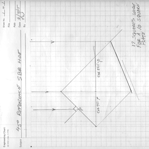
In this sketch of the set up, the expanded and collimated laser beam is coming from the left, as is usual in optical schematics.
The lowermost ray is incident on the center of the holoplate at the requisite reference angle of 45°. There is a ray above it which just misses the holoplate, but is reflected by a front surface mirror to arrive along the normal to the bottommost portion of the plate. Positioning the mirror this far back eliminates any shadows cast by the recording material which would attenuate this beam and add its scatter to this beam, possibly making it not a true point source but something on the diffusely scattering side, especially at the bluer wavelengths.
If you are having a hard time reading the printing on the sketching, rollover it with your mouse and the image will rotate into something more legible. The point of the trigonometry is to determine the size of the expanded beam needed to fill the holoplate from both sides, and the conclusion is that the beam’s diameter needs to be about 1.7X the width of the plate, although the height of the plate plays into the practical implementation.
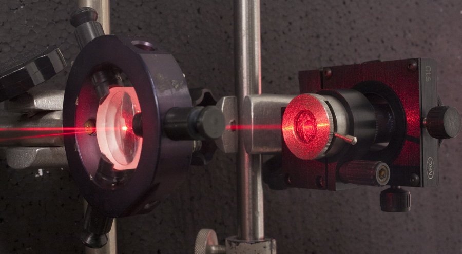
Here is the physically implemented set up:
Although this is a single beam set up, the beam balance ratio can still be controlled. Laser beams’ profiles are not even but vary along the diameter in the well-known Gaussian distribution. This beam profile was translated across the holographic plate and “object” mirror by a long focal length negative lens before the spatial filter.
A simple silicon detector was positioned in the center of a piece of cardboard of the holoplate dimensions and measured the radiant flux on first one side and then the other.
The laser beam’s profile was shifted so that both sides read the same amount of light. The 45° incidence side was in the brighter center due to incident angle attenuation and reflection, and the beam along the normal which was not so affected used the weaker outer portion of the beam. There were gradients of flux out in the edges, but a 1:1 ratio was attained in the center of the holoplate.
Samples of holographic recording materials were positioned in the plateholder and exposed at a variety of energy levels, generally bracketing around the manufacturer's suggested exposure dose and plus and minus a photographic stop by half stops. For example, if the manufacturer claimed sensitivity of 600 microJoules per square centimeter, then the exposure series would go 300, 420, 600, 840, and 1200 microJoules per square centimeter, for full stop less, half stop less, recommended, half stop more, full stop more.
Then they were processed in what was deemed the best soups for the job. Not only should the processing deliver bright results, but there should be no distortion like shrinkage or expansion of the layer to change the replay color. This parameter was checked with a spectrometer. The processing for both of the materials tested gave the desired results.
To characterize diffraction efficiency, Iris Diaphragms were positioned to change the recording set up into an in situ interrogation set up.
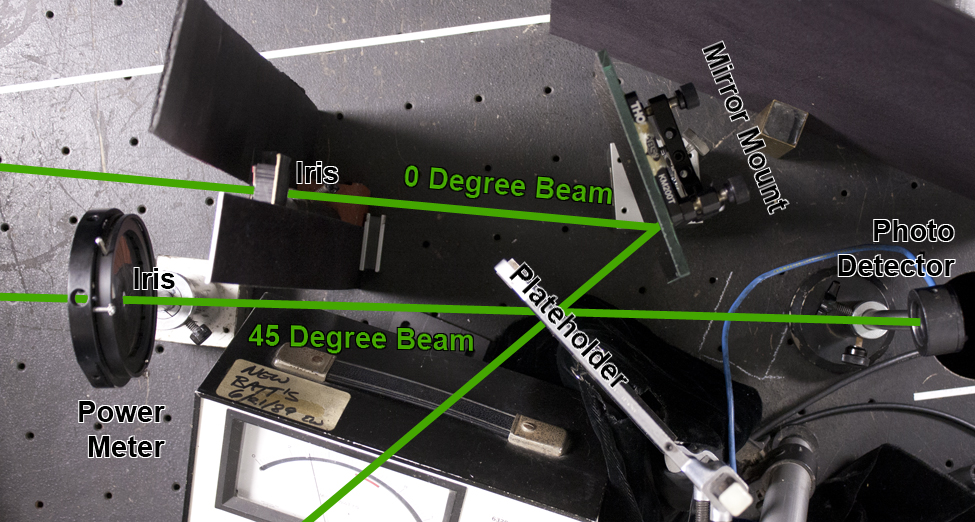
Iris diaphragms were positioned in the parts of the large spread beam corresponding to 45° direct incidence and 0° incidence by way of the mirror. The irises were translated in the beam so that their projections were centered on a piece of groundglass, with alignment guides, the size of the sample plates.
The size of the iris was chosen so that it would be large enough to sample a decent chunk of hologram to average out irregularities, and accommodate any ellipticizing of beams. The center of the plate is where the Beam Balance Ratio was measured to be unity, so it is the prime fillet of the hologram.
The aperture size was further refined so that the free space travelling light (no glass in the plateholder) would read full scale deflection on the Newport Model 820 Power Meter. Then the first order diffraction figure in the Excel SpreadSheet or table becomes the diffraction efficiency in percent. (Scale used on the meter is 10mW, but the cm2 suffix does not apply as the detector is underfilled.)
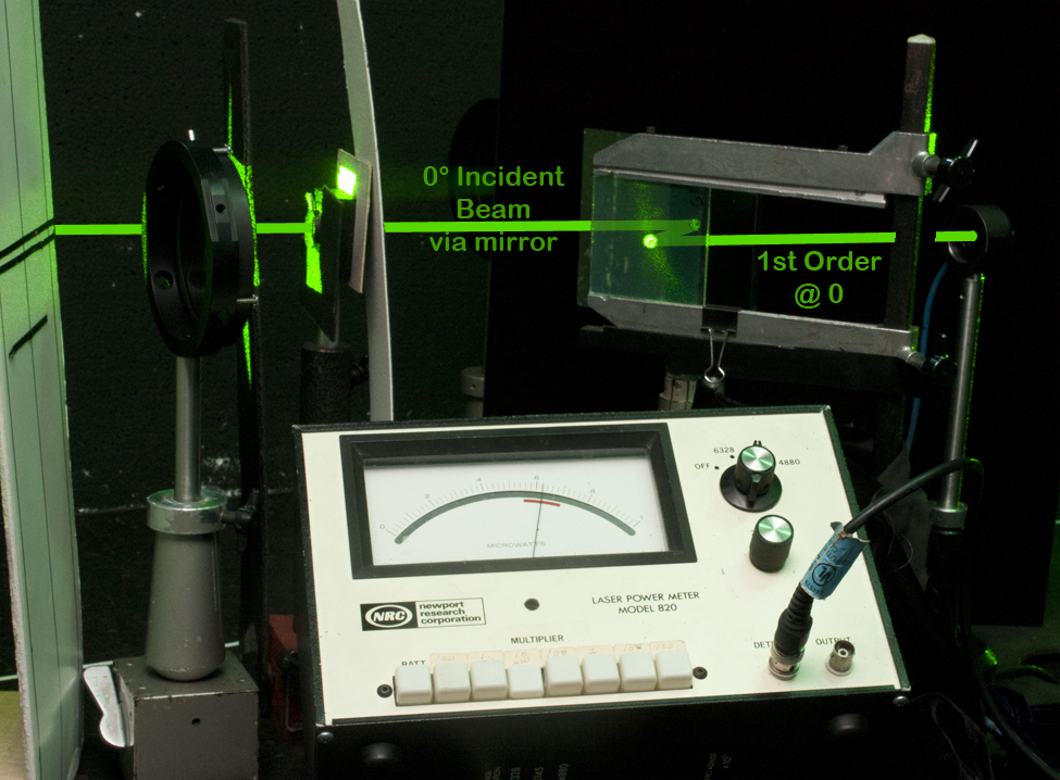
The detector position is changed for the replay beam at normal incidence. It is also the position where the 1st order from 45° incidence is measured.
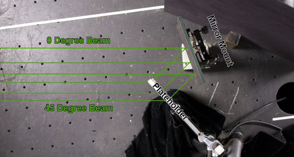
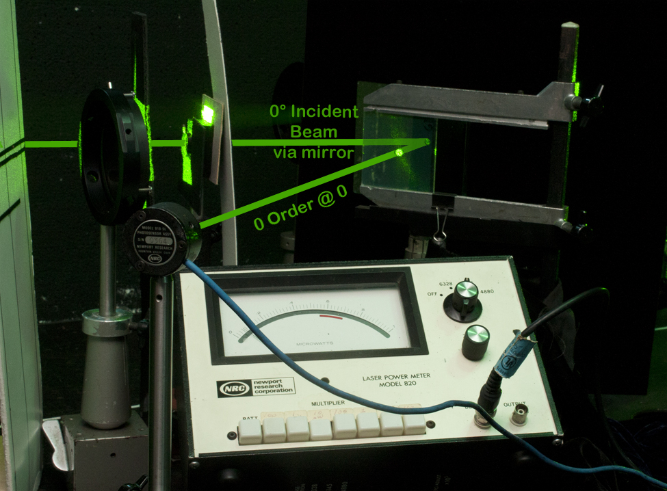
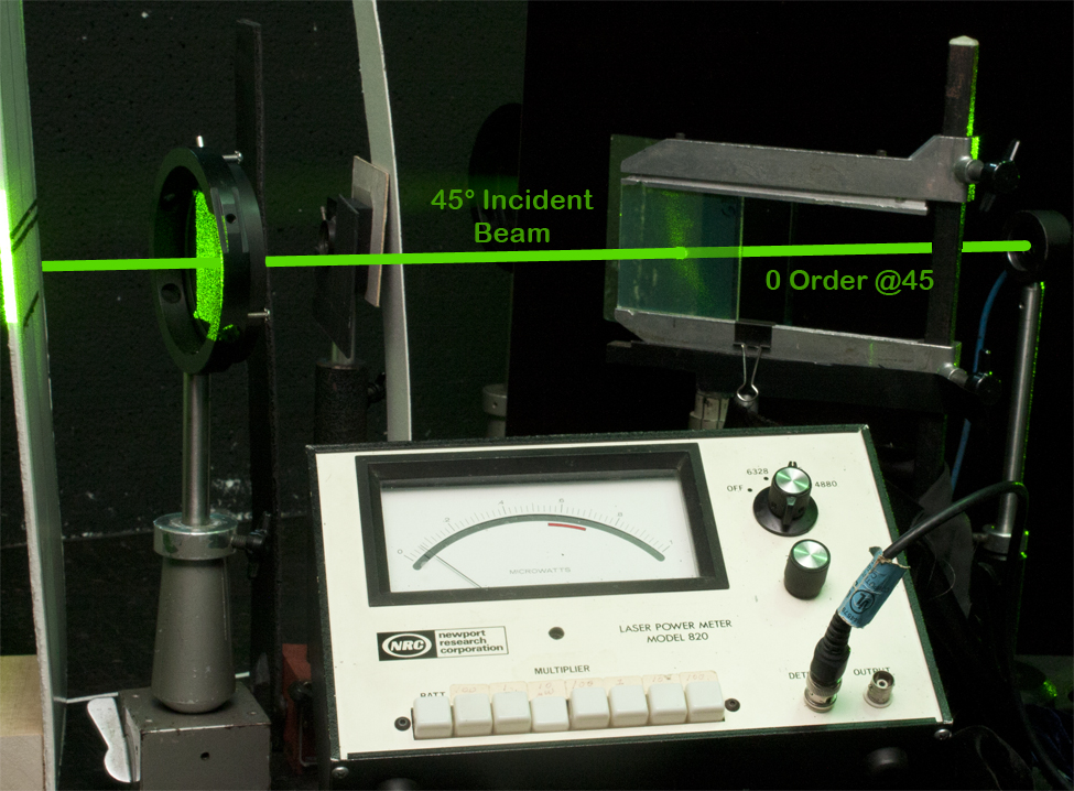
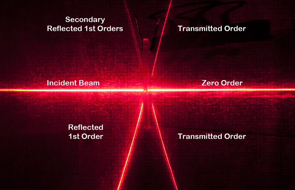
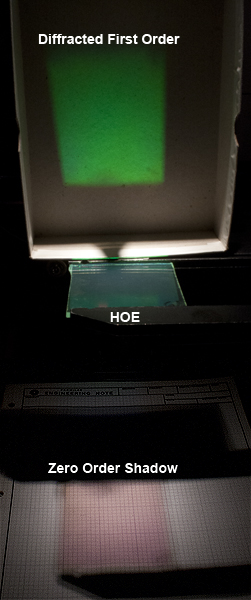
Similarly the detector position measuring the 0 order of the 45° incidence beam is the same place as the 1st order from 0° incidence. Shuttling the beam-blocking card between the two apertures allows for quick data intake at both detector positions.The four different measurements taken were the Zero Order Beams of both incident beams, and the diffracted First Order Beams of both of the Incident Beams, and are illustrated below. The beams in the images are captioned with the titles of the pertinent spreadsheet columns coming up.
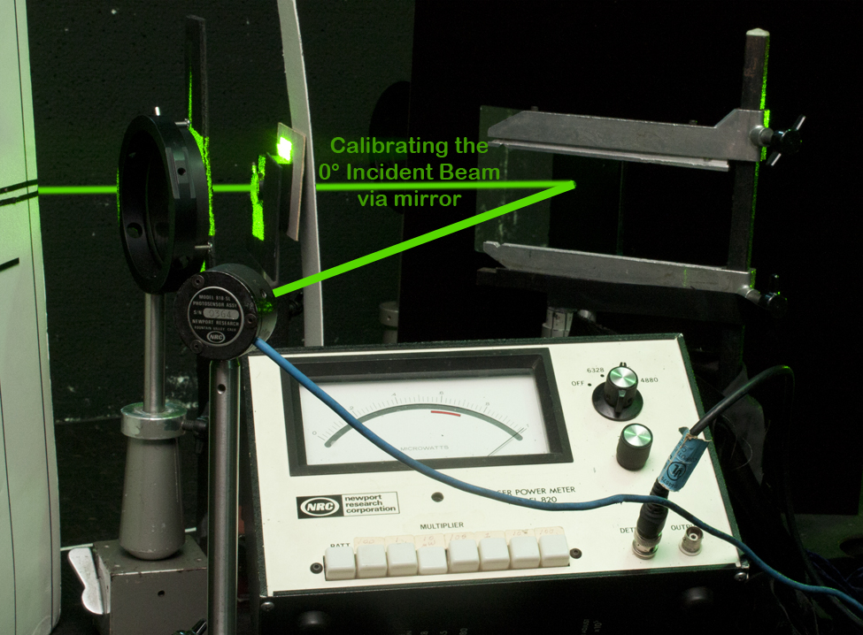
Here is the set up for measuring the 1st order at 0° incidence (by way of the mirror).
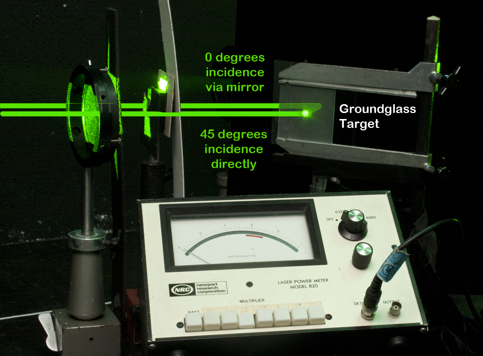
Here is how the 0 Order at 45° incidence was measured:
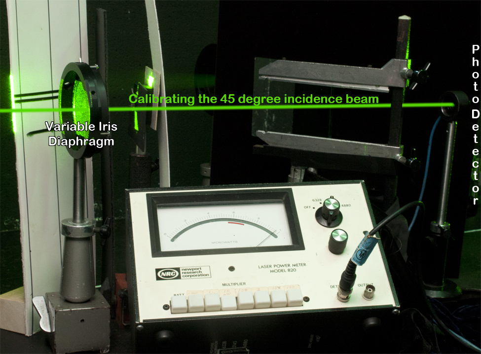
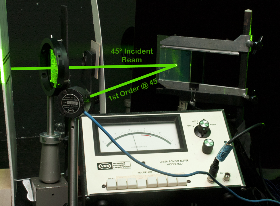
Here is how the 1st Order at 45° incidence was measured:
Here are tables for the test exposure series on Sphere-S GEO-3 plates at the various recording wavelengths, as measured in the above rig.
At 532 nm, 1’ development time, exposures in μJ/cm²:
SAMPLE # |
0 ORDER @ 0 |
1st ORDER @ 0 |
0 ORDER @45 |
1st ORDER @ 45 |
EXPOSURE |
59 |
22 |
44 |
18 |
40 |
1600 |
60 |
8 |
56 |
8 |
50 |
2200 |
61 |
8 |
64 |
8 |
48 |
3200 |
62 |
6 |
52 |
6 |
44 |
4500 |
Since 100 units of light were available without the hologram in position, the 1st order values are directly translatable into diffraction efficiency percent! (If you want to take into account the effect of reflection off the surface of the hologram, multiply the first order results by 1.04)
The sum of the 0 and 1st orders do not add up to 100, so there is about a quarter of the incident light lost due to spurious holographic images and scatter. For instance, for sample #61, 8% of the incident light passed through as the Zero Order at Zero degrees incidence, plus 64% diffracted into the First Order at the same time, leaving 28% of the light unaccounted for. Here is a ray trace of some of the spurious images for a similarly recorded grating at 633 nm.
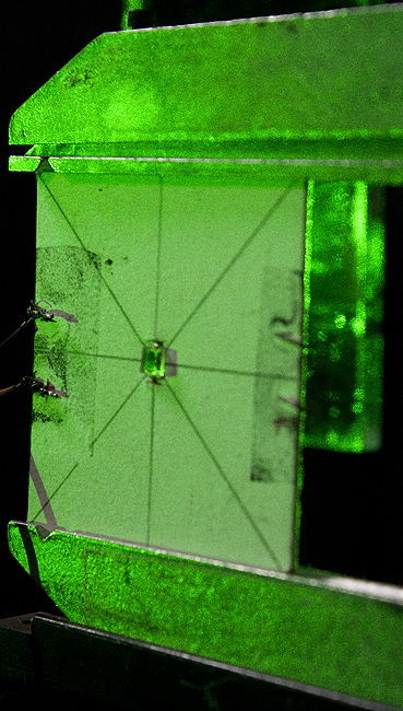
During this project I had access to an Ocean Optics Jaz spectrometer. The hologram was interrogated by it in this set up:
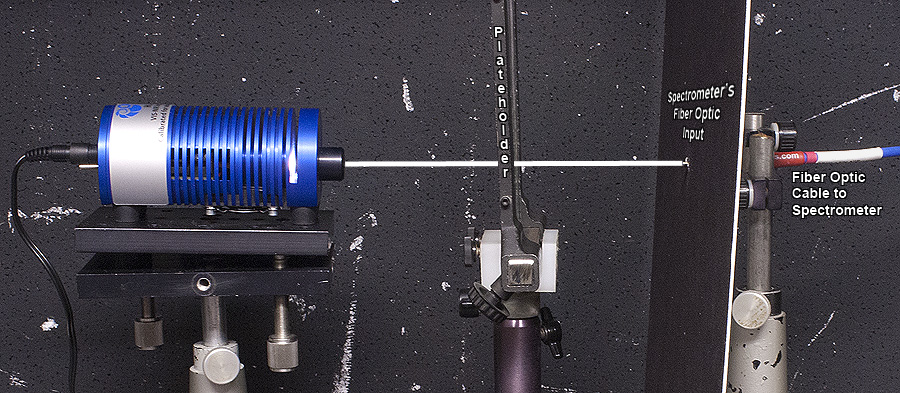
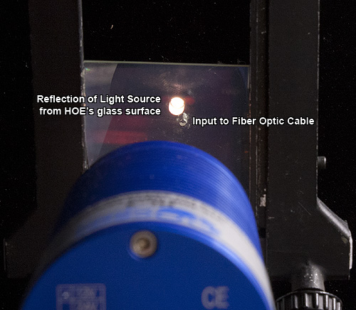
A calibrated black body radiator, Ocean Optics HL-3, feeds light into the collecting fiber optic, which delivers it to the spectrometer housing. The hologram is replayed at normal incidence, which is an angle that is consistently repeatable, by looking over the shoulder of the light source and verifying that the reflection of the output of the black body source is coincident on the fiber optic’s input.
The plate could be translated in grooved holder to map out regions of diffracted interest. The holographic plateholder could rock the hologram to control its y-axis pitch, and a Newport Rotation Stage could rotate the x-axis’s yaw, useful for measuring changes in the replay angle. Roll was not an issue.
The data was taken in the Jaz’s Transmission Mode, which measures the depletion of the various wavelengths compared to a previously calibrated baseline at the top of the graph, which is marked 100. Here are scans of the samples from the table above, and the 0 order depletion in the scan's table is in good agreement with the per cent transmission!
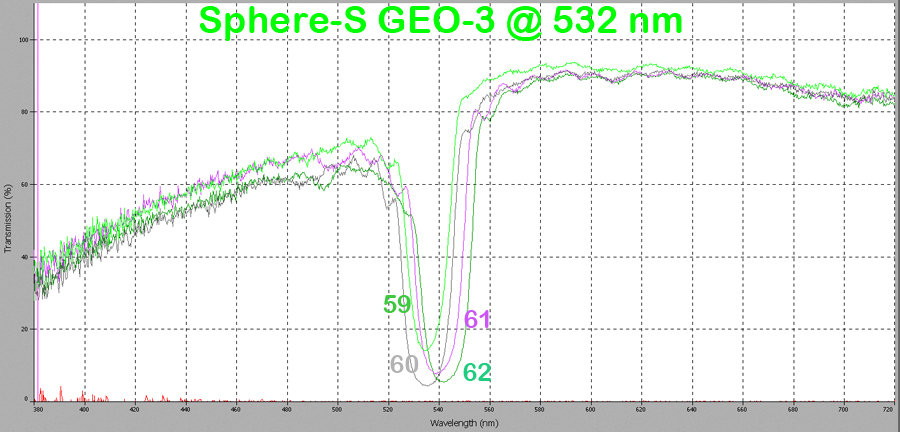
The depth of these scans does not necessarily indicate absolute diffraction efficiency. #60 in the scan above has the deepest dip, looking to be transmitting only about 6%, but the missing 94% is not seen in the diffracted first order in the table above, only 56%. The rest is lost due to spurious images as shown above or scatter.
The Rayleigh scatter equation is roughly graphed in the above. When the instrument is set up and calibrated, its parameters are adjusted so that the black body radiator’s curve is normalized to the 100% horizontal scale line. But the transmission curve of the hologram has the shape of Lord Rayleigh's 4th order polynomial that takes wavelength to that power! More light is lost to scatter at the blue end of the spectrum. One wishes that there were a way to measure grain size using this artifact.
The usefulness of these scans is in checking the replay wavelength and bandwidth. For the most part these samples retained the fringe spacing of the recording wavelength as evidenced by the dip at approximately 532 nm. Each sample number was a separate plate, so the wavelength variation may be due to operator error when lading the plate in recording or replay.
These samples are so efficient that their projected shadows under white light have a decidedly magenta cast, as could be deduced from the above graph!
Same measurements for the exposure series recorded at 458 nm, 1’ development time.
SAMPLE # |
0 ORDER @ 0 |
1st ORDER @ 0 |
0 ORDER @45 |
1st ORDER @ 45 |
EXPOSURE |
64 |
6 |
34 |
3 |
40 |
1600 |
65 |
10 |
62 |
5 |
60 |
2200 |
66 |
10 |
58 |
8 |
56 |
3200 |
67 |
12 |
44 |
10 |
38 |
4500 |
Yes, Sample #65 is exhibiting an honest 60+% diffraction efficiency!
Scan of the bandwidth and wavelength accuracy of the above:
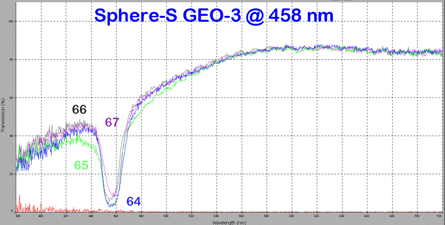
Replay wavelength is well-preserved!
Here is the red data:
SAMPLE # |
0 ORDER @ 0 |
1st ORDER @ 0 |
0 ORDER @45 |
1st ORDER @ 45 |
EXPOSURE |
46 |
28 |
40 |
28 |
44 |
2200 |
47 |
14 |
44 |
20 |
40 |
3200 |
48 |
10 |
30 |
28 |
28 |
4500 |
Plus spectral:
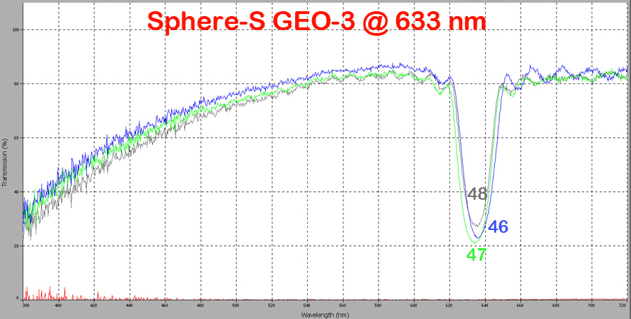
Surprisingly, diffraction efficiency of the red exposures is slightly less than the shorter wavelengths. Conventional wisdom would say that red recording has lower spatial frequency and less scatter, so it should be better. Perhaps the He-Ne (Uniphase 1145P) does not have as good coherence as the DPSS green and blue lasers (Coherent Compass 315M-100 and Melles Griot BLD-605, respectively)?
ROUND TWO:
More exposure tests were run at 532 nm on Ultimate Holography's Ultimate U04 panchromatic material. The exposure series was bracketed around the suggested 600 microJoules per centimeter squared by full stops.
SAMPLE # |
EXPOSURE |
0 ORDER @ 0 |
1st ORDER @ 0 |
0 ORDER @ 45 |
1st ORDER @ 45 |
87 |
150 |
58 |
18 |
58 |
18 |
88 |
300 |
38 |
34 |
40 |
38 |
89 |
600 |
18 |
54 |
20 |
58 |
90 |
1200 |
18 |
54 |
18 |
62 |
91 |
2400 |
28 |
22 |
28 |
41 |
Replay wavelength:
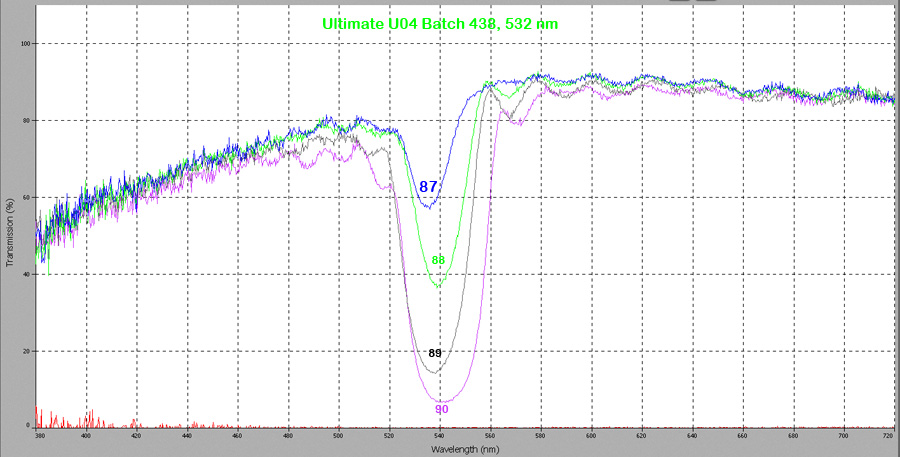
There is a curious broadening of the replay bandwidth with exposure.
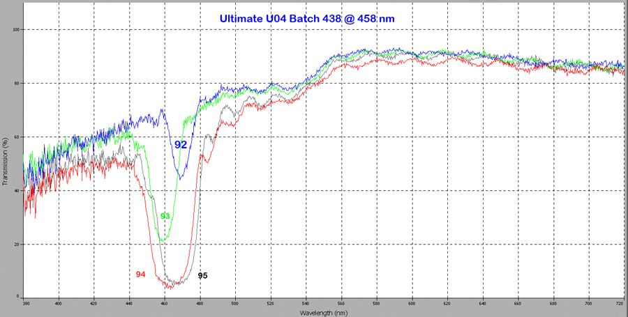
Here is what happens with the blue:
SAMPLE # |
EXPOSURE |
0 ORDER @ 0 |
1st ORDER @ 0 |
0 ORDER @ 45 |
1st ORDER @ 45 |
92 |
150 |
72 |
2 |
66 |
2 |
93 |
300 |
18 |
42 |
22 |
42 |
94 |
600 |
4 |
58 |
20 |
66 |
95 |
1200 |
6 |
50 |
7 |
66 |
96 |
2400 |
8 |
50 |
6 |
56 |
And its replay color characteristics:
And since you asked, here is the red diffraction data:
SAMPLE # |
EXPOSURE |
0 ORDER @ 0 |
1st ORDER @ 0 |
0 ORDER @ 45 |
1st ORDER @ 45 |
97 |
150 |
75 |
12 |
80 |
10 |
98 |
300 |
36 |
44 |
40 |
46 |
99 |
600 |
20 |
60 |
24 |
60 |
100 |
1200 |
25 |
56 |
25 |
60 |
101 |
2400 |
26 |
40 |
40 |
36 |
Plus the spectral scan:
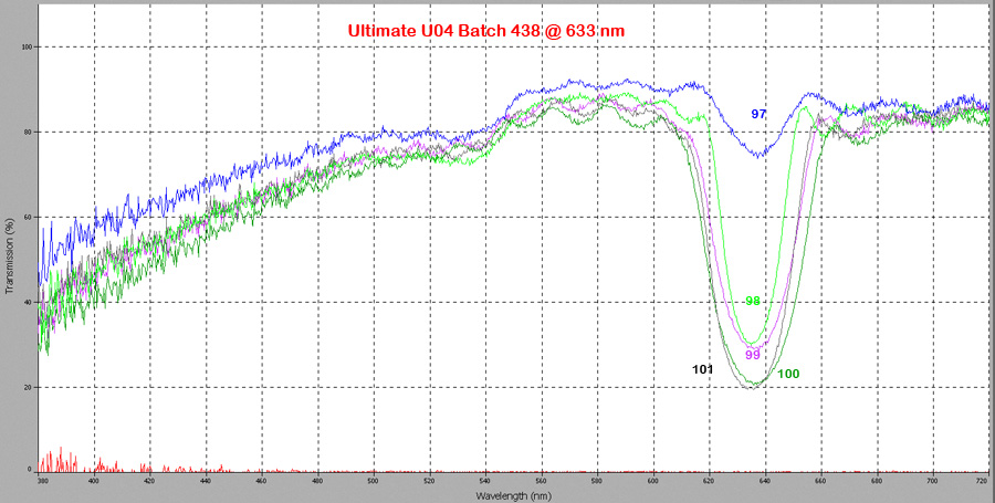
Again the red doesn't have the same efficiency and zero order extinction as the blue and green exposures. This must be a good case for acquiring a Single Longitudinal Mode laser! But that shouldn't stop anyone from shooting a hologram with all three wavelengths!
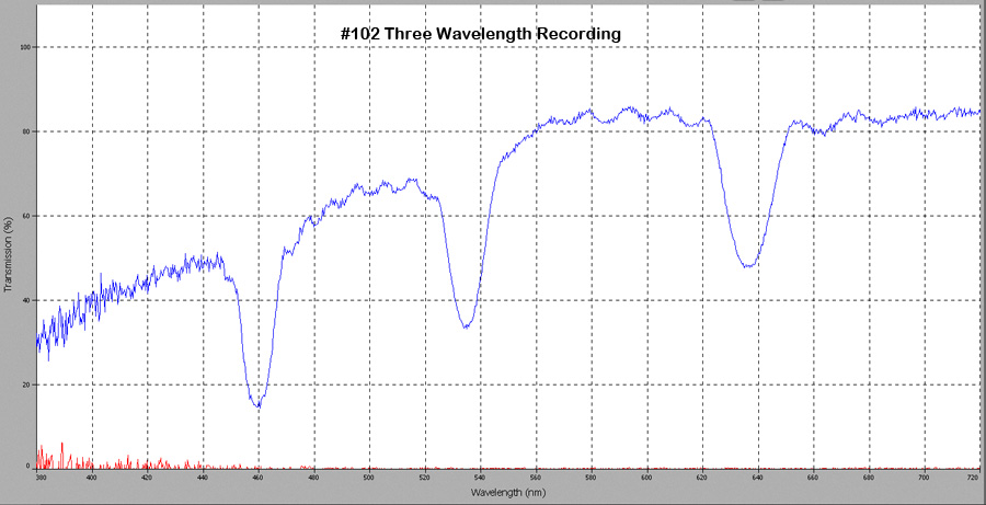
SAMPLE # |
EXPOSURE |
0 ORDER @ 0 |
1st ORDER @ 0 |
0 ORDER @ 45 |
1st ORDER @ 45 |
102 |
300 R |
52 |
30 |
56 |
28 |
102 |
300 G |
35 |
38 |
38 |
34 |
102 |
300 B |
18 |
46 |
16 |
32 |
And the scan of the "white" replay:
CONCLUSIONS:
The Single Beam Reflection Hologram of a Mirror technique can record some useful Holographic Optical Elements, if for no other reason than to duplicate this experiment for measuring diffraction efficiency of most any holographc recording material. Although a collimated beam was used for this set up, it does not necessarily need to be so.
A calibrated power meter is not necessary either, although it helps when publishing exposure data that might conceivably be duplicated in other labs. But the determination of the diffraction efficiency can be done with any photo detector, like a silicon cell or photo resistor simply plugged into a VOM, as it is simply the ratio of diffracted beam to incident beam.
Not everyone happens to have a spectrometer at their home lab, but if you got 'em, smoke 'em. It is very useful for seeing the replay bandwidth of the HOE, and can be applied to any reflection hologram, image or Optical Element. There is a real danger for using the transmission curve of the sample for evaluating diffraction efficiency, althought they are related, but some manufacturer's do use them in their advertising!